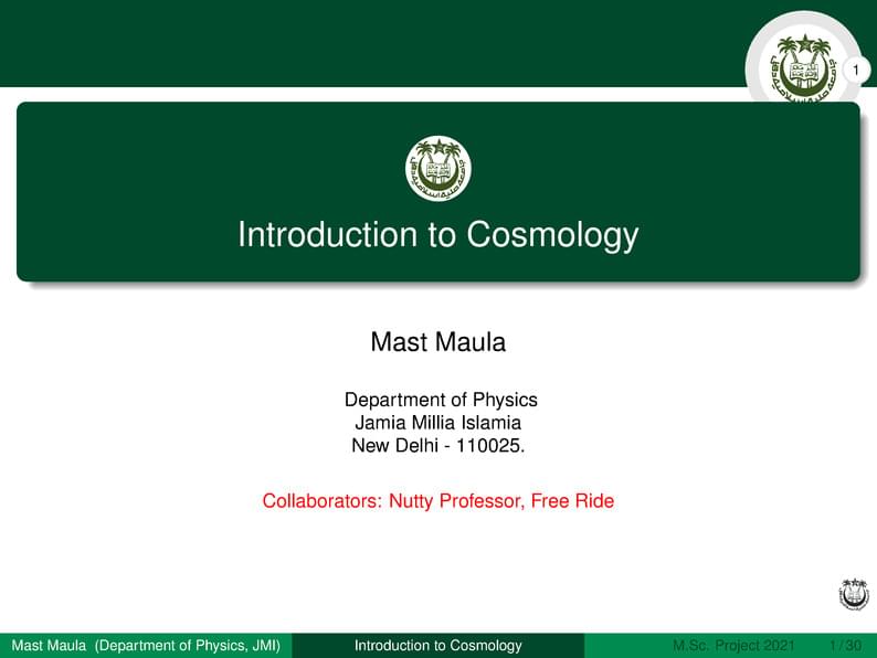
JMI beamer template
Author:
Tabish
Last Updated:
5 years ago
License:
Creative Commons CC BY 4.0
Abstract:
Latex beamer template for a presentation

\begin
Discover why over 25 million people worldwide trust Overleaf with their work.

\begin
Discover why over 25 million people worldwide trust Overleaf with their work.
\documentclass[xcolor=dvipsnames]{beamer}
%\setbeamercovered{invisible}
\setbeamercovered{transparent}

\mode<presentation>
{
  \usetheme{JMI}
  \useoutertheme{JMIdial} % Comment this out if you don't want the counter dial
%  \useoutertheme[rotationcw]{JMIdial} % Clockwise rotation, instead of CCW
}

\usepackage[english]{babel}
\usepackage{wrapfig}
\usepackage{animate}
\usepackage[latin1]{inputenc}
\usepackage{times}
\usepackage[T1]{fontenc}
\usepackage{color, colortbl}
\usepackage{tikz}
\usetikzlibrary{arrows,shapes}
\title[Introduction to Cosmology] % (optional, use only with long paper titles)
{Introduction to Cosmology}

%%\subtitle
%%{Include Only If Paper Has a Subtitle}

\author[Mast Maula] % (optional, use only with lots of authors)
{Mast Maula}
% - Give the names in the same order as the appear in the paper.
% - Use the \inst{?} command only if the authors have different
%   affiliation.

\institute[Department of Physics, JMI] % (optional, but mostly needed)
{
%%  \inst{1}%
  Department of Physics\\
  Jamia Millia Islamia\\
  New Delhi - 110025.
  }
% - Use the \inst command only if there are several affiliations.
% - Keep it simple, no one is interested in your street address.

\date[M.Sc. Project 2021] % (optional, should be abbreviation of conference name)
{\textcolor{red}{\scriptsize Collaborators: Nutty Professor, Free Ride}}
% - Either use conference name or its abbreviation.
% - Not really informative to the audience, more for people (including
%   yourself) who are reading the slides online

\subject{Cosmology}
% This is only inserted into the PDF information catalog. Can be left
% out.

% Delete this, if you do not want the table of contents to pop up at
% the beginning of each subsection:
\AtBeginSection[]
{
\begin{frame}<beamer>
  \frametitle{Outline}
  \tableofcontents[currentsection,currentsubsection]
  % You might wish to add the option [pausesections]
\end{frame}
}

% If you wish to uncover everything in a step-wise fashion, uncomment
% the following command:

%\beamerdefaultoverlayspecification{<+->}

\newcommand{\op}{\boldsymbol}
\newcommand{\ua}{\uparrow}
\newcommand{\da}{\downarrow}
\newcommand{\red}{\textcolor{red}}
\newcommand{\blue}{\textcolor{blue}}
\newcommand{\green}{\textcolor{OliveGreen}}
\begin{document}

\begin{frame}
  \titlepage
\end{frame}

\begin{frame}
  \frametitle{Outline}
  \tableofcontents
  % You might wish to add the option [pausesections]
\end{frame}

\section{Homogeneous and Isotropic Model}
\begin{frame}
\frametitle{Homogeneous and Isotropic Model}

{\bf Homogenity:} Means that universe looks the same at each point.
\vskip 3mm

{\bf Isotropy:} Means that universe looks the same in all directions.
\vskip 3mm

These are two important properties of space which are independent of each
other. But isotropy at each point implies homogenity also.
\vskip 3mm
\pause

{\bf Cosmological principle:} {\em Universe is homogeneous and isotropic at
any given cosmic time.}
\vskip 3mm

The cosmological principle is supported by the
observational evidence that the universe becomes smooth at large scales.
The cosmological principle presents the idealized picture of the universe.
The departure from homogenity and isotropy is extremely important which led
to the structure formation in the universe.
\end{frame}


\begin{frame}
\frametitle{Hubble's law}
\begin{wrapfigure}{r}{2cm}
\resizebox{!}{2cm}{\includegraphics[width=2cm]{cosmofig1.png}}
\end{wrapfigure}
We examine the motion of matter in a coordinate system in
which it is at rest at the origin. We now ask for the velocity
dstribution consistent with homgenity and isotropy.

Hubbles law:
\begin{equation}
\vec{v} = H(t) \vec{r}
\end{equation}
Velocity field (1) is isotropic at $O$. Let us verify that (1)
holds for any observer situated at a point $A$, The observer at $A$ is in
motion with respect to $O$.

\begin{wrapfigure}{r}{2cm}
\resizebox{!}{2cm}{\includegraphics[width=2cm]{cosmofig2.png}}
\end{wrapfigure}
$$ \vec{r}' = \vec{r} - \vec{r}_A . $$
So,
\begin{eqnarray}
\vec{v}' &=& \vec{v} - \vec{v}_A = H\vec{r} - H\vec{r}_A \nonumber\\
\vec{v}' &=& H (\vec{r} - \vec{r}_A) \nonumber\\
\vec{v}' &=& H \vec{r}' \nonumber
\end{eqnarray}

Therefore, velocity distribution (1) is homogeneous and isotropic.
\end{frame}

\begin{frame}
\frametitle{Local expansion}
The distance between two arbitrary points changes as
$$ \frac{d\vec{r}_{AB}(t)}{dt} = H(t) \vec{r}_{AB} $$
Therefore,
$$ \vec{r}_{AB}(t) = \vec{r}_{AB}(t_0) \exp\left(\int_{t_0}^tH(t')
dt'\right) $$
{\bf Remark:} The dynamics will be decided by $H(t)$.\\
 If $H(t)=const.$, then
$$ \vec{r}_{AB}(t) = \vec{r}_{AB}(t_0) e^{(t-t_0)H}$$
\end{frame}

\begin{frame}
\frametitle{Evolution of density}
\begin{wrapfigure}{r}{4cm}
\resizebox{!}{4cm}{\includegraphics[width=4cm]{cosmofig3.png}}
\end{wrapfigure}
$$      \rho = {M \over {4\pi\over3}R^3}$$
Differentiating w.r.t. time
$${d\rho(t)\over dt} = -{3M\over[{4\pi\over3}R^4]} {dR\over dt} $$
But $dR/dt = v = HR$. Therefore,
$$ {d\rho(t)\over dt} = -{3M\over[{4\pi\over3}R^3]}H = -3\rho H $$
\begin{equation}
{d\rho\over dt} = -3\rho H
\end{equation}
\end{frame}

\begin{frame}
The last can also be obtained from continuity equation
$$ {\partial\rho\over\partial t} = - \vec{\nabla}\cdot (\rho \vec{v}) $$
$\rho$ - function of time alone:
\begin{equation}
{\partial\rho\over\partial t} = \rho H \vec{\nabla}\cdot\vec{r} = -3\rho H
\end{equation}
$$	{\partial\rho\over\partial t} = {d\over dt}\rho $$
Homogeneity and isotropy is a preserved property in time.
\end{frame}

\section{Evolution Equation}

\begin{frame}
\begin{wrapfigure}{r}{4cm}
\resizebox{!}{4cm}{\includegraphics[width=4cm]{cosmofig4.png}}
\end{wrapfigure}
The acceleration of a particle with mass $m$ due to the gravitational force
of $M$ is given by:
$$ {d^2R(t)\over dt^2} = {-GM\over R^2(t)}  $$
$$ {d^2R(t)\over dt^2} = {d\over dt}(HR) = H{dR\over dt} + R{dH\over dt} = H^2R + R{dH\over dt} $$
$$ {dH\over dt} = - {GM\over R^3} - H^2 $$
\begin{eqnarray}
\frac{dH}{dt} = -H^2 - {4\pi\over 3}G\rho
\end{eqnarray}

{\bf Remark:} If $H=const$, eqn (4) is inconsistent. Infact $H=const$
(with ${dh\over dt}={\ddot{R}\over R} - H^2$) would imply $\ddot{R}(t)>0$,
which cannot come from eqn (4).
\end{frame}

\begin{frame}
{\bf Friedman Equation:} Multiply eqn (3) by $dR(t)/dt$:
$$ {dR\over dt}\left({d^2R\over dt^2}\right) = -{GM\over R^2} {dR\over dt} $$
$$ {1\over 2}{d\over dt}\left({dR\over dt}\right)^2 ={d\over dt}\left({GM\over R}\right) $$
$$ {d\over dt}\left[{1\over 2}\left({dR\over dt}\right)^2 -{GM\over R}\right]=0 $$
\begin{equation}
\boxed{{1\over 2}\left({dR\over dt}\right)^2 -{GM\over R}=A=const }
\end{equation}
\[ M = \frac{4}{3}\pi\rho R^3 \]

{\bf Determining the constant $A$}

\{$t_0$, $\rho_0$ \} present epoch and select a value of $R=R_0$ at $t=t_0$
for the sphere.
\begin{eqnarray}
A &=& {1\over 2}\left({dR\over dt}\right)^2_{t=t_0} -\frac{4}{3}\pi GR_0^2\rho_0
\nonumber\\
 &=& \frac{1}{2}H_0^2R_0^2 -\frac{4}{3}\pi GR_0^2\rho_0\nonumber
\end{eqnarray}
\begin{equation}
\boxed{\left({dR\over dt}\right)^2 = \frac{8\pi G}{3}\rho R^2
- \frac{8\pi G}{3}R_0^2\left[\rho_0 - \frac{3H_0^2}{8\pi G}\right] }
\end{equation}
This is called Freidman equation. From continuity equation
\[ \boxed{ \rho(t) = \frac{\rho_0R_0^3}{R^3} }  \]
\end{frame}

\begin{frame}
\frametitle{General character of the solution of (6)}
At present, $\frac{dR}{dt} > 0$ implies that $R$ was smaller in the past,
but $\frac{8\pi G}{3}\rho R^2$ was larger, so $\frac{dR}{dt}$ was larger
in the past:
\[ \boxed{ R(t_0) = 0,~~~~~~\left.\frac{dR}{dt}\right|_{t=t_0} = +\infty
~~~~~~~~t=t_0 } \]
Explanation

\fbox{ $R\ge 0$ by definition, $\ddot{R}(t)<0$, $\rho >0$ }\\
Hence $R(t)$ was smaller and smaller as we go into past deeper and deeper,
and $dR/dt$ becomes larger and larger. Consequently, there was an epoch,
say $t=0$, when
\[ R(t=0) = R(0) = 0~~~~~~~~~\left.\frac{dR}{dt}\right|_{t=0} = \infty \]
\end{frame}

\begin{frame}
\frametitle{Critical density}
\begin{wrapfigure}{r}{4cm}
\resizebox{!}{4cm}{\includegraphics[width=4cm]{cosmofig5.png}}
\end{wrapfigure}
The prediction of the future depends upon the sign of $[\rho_0-3H_0/8\pi G]$
or how the present density compares with the critical density $\rho_c$:
\[ \rho_c = \frac{3H_0^2}{8\pi G} \]
We also defined the dimensionless density parameter $\Omega_0$:
\[ \Omega_0 \equiv \frac{\rho_0}{\rho} = \frac{8\pi G\rho_0}{3H_0^2} \]
\end{frame}


\begin{frame}
\frametitle{Classification of the solution}
\begin{columns}
\column{8cm}
\begin{enumerate}
\item{I} $\rho_0 > \rho_c$ The second term in eqn (6) is positive. As $R$
increases, the first term decreases and eventually becomes equal to the
second term at a particular time. The RHS of eqn (6) then vanishes and
expansion ceases, and contraction begins.
\pause

\item{II} $\rho_0 < \rho_c$  RHS of equation (6) is positive, leading to
expansion forever.\\
As $t\to\infty$, $R\to\infty$
\[ \left.\frac{dR}{dt}\right|_{t=\infty}=\left[\frac{8\pi G}{3}R_0^2
(\rho_c-\rho)\right]^{1/2} \]
\pause

\item{III} $\rho_0 = \rho_c$ Expansion continues without bound.
\end{enumerate}
\column{4cm}
\includegraphics[width=4cm]{cosmofig6.png}
\end{columns}
\end{frame}


\begin{frame}
\frametitle{Maximum Age Estimate}
$t=0$, $R=0$. Suppose the expansion rate is constant and given by the present
value of Hubble parameter,
\[ R(t_0) \equiv R_0 = \left(\frac{dR}{dt}\right)_{t=0}t_0 = H_0R_0t_0 \]
\[ \boxed{t_0 = \frac{1}{H_0}}~~~~~~\boxed{ T_0 \simeq h^{-1}9.8\times 10^9
years} \]
\[ H_0 \simeq 100 km s^{-1}mpc^{-1}~~~h\simeq 1-0.5~~~~
t\simeq 9.8\times 10^9h^{-1} years \]
\[ 0.37 < H_0t_0 < 1.47 \]
\end{frame}

\section{Solutions of Evolution Equation}

\begin{frame}
\frametitle{Solutions of Evolution Equation}
$\rho_0=\rho_c$ or $\Omega_0=1$

\[ \left(\frac{dR}{dt}\right)^2 = \frac{8\pi G}{3}\rho R^2
~~~~~~~~~~~~\boxed{ \rho(t) = \frac{\rho_0}{R^3}R_0^3} \]

\[ \left(\frac{dR}{dt}\right)^2 = \frac{8\pi G}{3}\frac{\rho_0 R_0^3}{R}
~~~~~~~~~~~~ dR R^{1/2} = const. dt \]
\[ R(t) = R(t=0)(t/t_0)^{2/3} ~~~~~~~\Rightarrow
\boxed{ R_0\left(\frac{t}{t_0}\right)^{2/3} = R(t)} \]
\[ R(t) \propto t^{2/3} \]
\[ \dot{R}(t) \propto \frac{2}{3}t^{-1/3}
~~~~\Rightarrow ~~~~ \frac{\dot{R}(t)}{R} = \frac{2}{3}\frac{1}{t}\]
\end{frame}

\begin{frame}
Therefore, $t_0 = \frac{2}{3}\frac{1}{H_0}$.
\[ \rho(t) = \frac{\rho_0 R_0^3}{R^3(t)}=\frac{\rho_0R_0^3}{R_0^3(t/t_0)^2}
 = \frac{3H_0^2}{8\pi Gt^2} t_0^2 =\frac{3H_0^2}{8\pi Gt^2}\frac{4}{9}
\frac{1}{H_0^2} = \frac{1}{6\pi Gt^2}\]
\[ \boxed{\rho(t) =  \frac{1}{6\pi Gt^2} } \]
\end{frame}

\begin{frame}
\frametitle{Pressure corrections: Relativistic effects}
\begin{equation}
\frac{\partial\rho}{\partial t} + 3H\left(\rho + \frac{P}{c^2}\right) = 0
\end{equation}

\begin{equation}
\frac{\ddot{R}}{R} = \frac{-4\pi G}{3}\left(\rho + \frac{P}{c^2}\right)
\end{equation}

\begin{equation}
\frac{\dot{R}^2}{2} - \frac{4\pi G}{3}R^2\rho = A
\end{equation}
\pause

\underline{\bf Consistency check:} Differentiating (9), we get
\[ \dot{R}\ddot{R}-\frac{4\pi G}{3}R^2\dot{\rho} - \frac{4\pi G}{3}\times 2
\times\rho\dot{R}R = 0 \]
$\dot{R} = HR$ lead to
\[ \boxed{
\frac{\ddot{R}}{R} = \frac{-4\pi G}{3}\left(\rho + \frac{P}{c^2}\right) }\]
System (7), (8) and (9) are consistent.
\end{frame}


\begin{frame}
\frametitle{Case of Radiation Domination}
{\bf Equation of State:} Out of the eqs (7), (8) and (9), only two are
independtent.
Eq. (9) can be obtained from (7) and (8). These eqs can be solved and $\rho(t)$, $R(t)$ can be uniquely determined provided the {\em equation of state}
(= relation between $\rho$ and $P$) is given. This relation, in simple cases,
can be written as
\[ P = \omega\rho c^2,~~~~~~~~~~~~~~~~~
\omega = \left\{
\begin{array}{ll}
0 & Dust\\
\frac{1}{3} & Radiation\\
-1 & Cosmological~constant\\
\end{array} \right. \]

$\omega=\frac{1}{3}$, $\rho_0=\rho_c$

\[ \frac{\partial\rho}{\partial t} + 3H\left(\rho+\frac{P}{c^2}\right)=0
~~~~~\Rightarrow~~~~~~\frac{\partial\rho}{\partial t} +4H\rho = 0 \]
\[ \boxed{ \rho(t) = \rho_0 \frac{R_0^4}{R^4(t)} } \]
\end{frame}

\begin{frame}
\[ \left(\frac{\dot{R}}{R}\right)^2 = \frac{8\pi G}{3}\rho
~~~~~~~~\Rightarrow~~~~~~ \dot{R}(t) \propto \frac{1}{R(t)} \]
\[ \boxed{ R(t) = R_0 \left(\frac{t}{t_0}\right)^{1/2} } \]
\[ H(t) = \frac{1}{2t}~~~~~~~~\Rightarrow~~~~~~~~~\boxed{t_0=\frac{1}{2H_0}} \]
\[ \rho(t) = \frac{3}{32\pi G} \frac{1}{t^2}  \]
\end{frame}

\section{Standard Form of Evolution Equations}

\begin{frame}
{\bf Comoving Coordinates:} These coordinates are are carried along with the
expansion. Since the expansion is uniform, the relation between the Physical
and Comoving Coordinates is given by
\[ \vec{r}(t) = a(t)\vec{x}~~~~~~~~~~~~~~~~~~ a(t) \rightarrow scale~factor \]
The uniformity of expansion is encoded in the scale factor.
\[ \left(\frac{dR}{dt}\right)^2 = \frac{8\pi G}{3}\rho R^2
-\frac{8\pi G}{3}R_0^2[\rho_0-\rho_c]  \]
Put $R(t) = a(t)x$
\[ \left(\frac{\dot{a}}{a}\right)^2 = \frac{8\pi G}{3}\rho -\frac{H}{x^2a^2} \]
\end{frame}

\begin{frame}
Let $Kc^2=\frac{A}{x^2}$ or $K=\frac{A}{x^2c^2}$. Dimensionally
\[ [K] = \frac{L^2}{T^2}\frac{1}{L^2\frac{L^2}{T^2}} = L^{-2} \]
\[ \left(\frac{\dot{a}}{a}\right)^2 = \frac{8\pi G}{3}\rho -\frac{Kc^2}{a^2} \]
Also, from (8)
\[ \frac{\ddot{a}}{a} = \frac{-4\pi G}{3}\left(\rho + \frac{3P}{c^2}\right) \]
Putting $c=1$
\[ \boxed{ \frac{\partial\rho}{\partial t} + 3H(\rho+P) = 0 } \]
\[\boxed{\left(\frac{\dot{a}}{a}\right)^2 = \frac{8\pi G}{3}\rho -\frac{K}{a^2} } \]
\[ \boxed{ \frac{\ddot{a}}{a} = \frac{-4\pi G}{3}(\rho + 3P) } \]
\end{frame}

\begin{frame}
\frametitle{Thermal History}
For $K=0$, $\rho_r(t) = \frac{3}{32\pi Gt^2}$
\[ \rho_r(t) = \alpha T^4  \]
\[\boxed{T = \left(\frac{3}{32\pi G\alpha}\right)^{1/4}t^{-1/2} } \]
\[ \boxed{T_K = 1.5\times 10^{10} t_{sec}^{-1/2} } \]

\[ \rho_r(t) \propto \frac{1}{a^4}~~~~~~\Rightarrow~~~~~~~~
 T(a) = T_0\left(\frac{a_0}{a}\right) \]
\end{frame}


\begin{frame}
\frametitle{Decoupling}
Decoupling takes place at a temperature equal to the binding energy of
Hydrogen atom.
\[ 3k_BT_d = 13.6 eV \]
\[ T_d = \frac{13.6 eV}{3k_B} \approx 5\times 10^4K~~~~(1eV \simeq 10^4K) \]

However, temperature in reality is much smaller than this
\[ T_d \simeq 3000 K~~~~~~~~\Rightarrow~~~~~~~~~~
\frac{a_0}{a_d}=\frac{3000}{T_0} \simeq 1000 \]
Since $T_K = 1.5\times 10^{10} T^{-1/2}$, decoupling time
\[ t_d = 10^{13}~sec \simeq 3\times 10^5~yrs. \]
\end{frame}

\begin{frame}

{\bf Remark:}
\begin{eqnarray}
\frac{\Omega_r}{\Omega_m} &\propto& \frac{1}{a} \nonumber\\
&=& \frac{\Omega_r^0}{\Omega_m^0}\frac{1}{a} \approx
\frac{4\times 10^{-5}}{\Omega_m^0}\frac{1}{a} \nonumber
\end{eqnarray}

\begin{eqnarray}
a_{eq} &\simeq& 2.4\times 10^4\Omega_0 \nonumber\\
t_{eq} &\simeq& 2.5\times 10^3\Omega_0^{-3/2}~years \nonumber
\end{eqnarray}
\end{frame}

\begin{frame}
\frametitle{Cosmological Constant}
Einstein introduced the {\em cosmological constant} to make the universe
static (later described by him as his ``biggest blunder'').
\[ H^2 = \frac{8\pi G}{3}\rho - \frac{K}{a^2} + \frac{\Lambda}{3} \]
\[ \rho_\Lambda = \frac{\Lambda}{8\pi G}~~~~~~~~~~~~
P_\Lambda = \frac{-\Lambda}{8\pi G} \]
$\Lambda > 0$ and $\rho$:  $H=0$
\[ a(t) \propto e^{\frac{\Lambda}{3}t} \]
\[ \frac{\ddot{a}(t)}{a(t)} = -\frac{4\pi G}{3}\left(\rho_\Lambda+3P_\Lambda
\right) = + \frac{8\pi G}{3}\rho_\Lambda  \]
$\ddot{a} > 0~~~\Rightarrow$ accelerated expansion. {\bf Inflation}
\end{frame}

\begin{frame}
\[ H^2 = \frac{8\pi G}{3}\rho - \frac{K}{a^2} + \frac{\Lambda}{3} \]
\[ 1 = \Omega_m + \Omega_\Lambda - \frac{K}{a^2H^2} \]
\[ \boxed{ \Omega_m + \Omega_\Lambda - 1 = \frac{K}{a^2H^2} }\]
\end{frame}

\begin{frame}
  \frametitle<presentation>{For Further Reading}

  \begin{thebibliography}{10}

  \beamertemplatebookbibitems
  % Start with overview books.

  \bibitem{narlikar}
    J. V. Narlikar
    \newblock {\em An Introduction to Cosmology}
    \newblock {(Cambridge University Press, 2002)}

  \bibitem{weinberg}
     Steven Weinberg
    \newblock {\em Cosmology}
    \newblock {(Oxford University Press)}

  \end{thebibliography}
\end{frame}

\end{document}