LaTeX templates and examples — Dynamic Figures
Recent

La bandera nacional de Malasia tiene un diseño muy semejante a la Bandera estadounidense, aunque su diseño se basa realmente en la bandera de la Compañía Británica de las Indias Orientales, en la que parece que también se inspiró aquella. Su diseño inicial fue creado por el arquitecto malayo Mohamed Hamzah quien envió a una competición en su país sus diseños en 1947. El público seleccionó su diseño entre los 373 que fueron enviados. Sin embargo, en 1963 fue rediseñada para tener en cuenta los nuevos estados del país, siendo adoptada el 16 de septiembre de ese año. Esta imagen se basa en la hoja de construcción de la página https://commons.wikimedia.org/wiki/File:Construction_sheet_of_Flag_of_Malaysia.svg de la cual se hizo la adaptación y los colores usados provienen del artículo de Wikipedia relacionado con la enseña nacional.
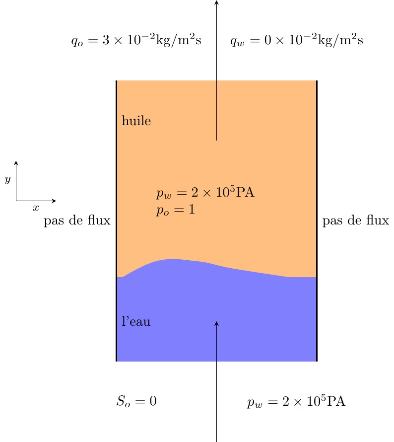
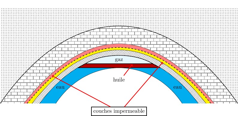
mechanics of fluid
We use \usepgfplotslibrary{fillbetween}

El 4 de Julio de 1949 un comité del gobierno de China solicitó al público diseños para la bandera nacional. Se presentaron 2992 diseños, los cuales fueron reducidos a 38 para llevarse a debate de la comisión. Uno de los diseños, presentado por Zeng Liansong (1917-1999) un habitante de Ruian, Wenzhou, provincia de Zhejiang, era similar a la bandera actual. Liansong incorporó el símbolo del partido comunista de China en el diseño de la bandera, representado por la estrella grande con una hoz y un martillo. El diseño de Zeng Liansong fue ligeramente modificado; se retiraron los emblemas de la estrella grande, y la bandera fue elegida oficialmente por el comité el 27 de septiembre de 1949 por voto unánime. Los detalles de diseño de la bandera actual se rigen por la ley aprobada el 28 de junio de 1990 y los colores por el estándar chino GB 12983-2004. El diseño y los colores se han tomado de la página http://www.vexilla-mundi.com/china_flag.html.
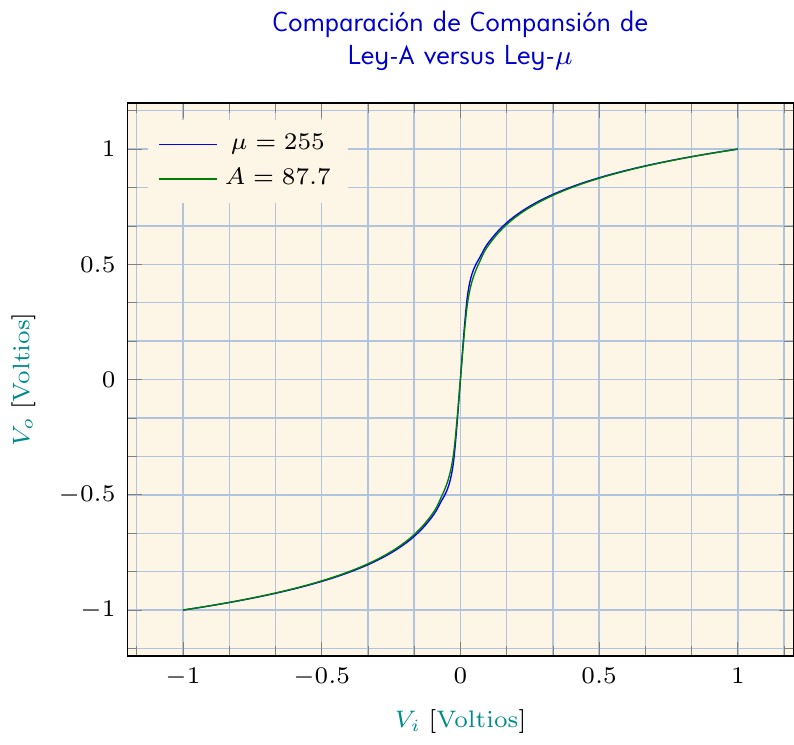
Este gráfico presenta las comparaciones de la compansión de una señal telefónica de entrada cuando es comprimida usando la Ley-A y la Ley-Mu tal se describen en la Recomendación G.711 de la Unión Internacional de Telecomunicaciones. De la gráfica se deduce que la compansión con ambas leyes no presenta mayores diferencias.
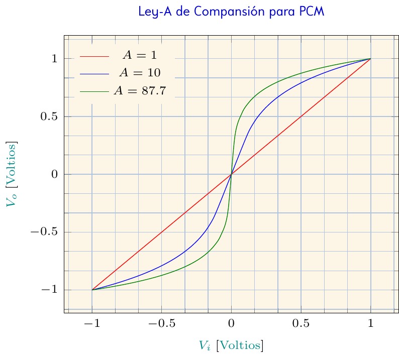
Este gráfico presenta las características de compresión de una señal telefónica de entrada cuando es comprimida usando la Ley-A tal como es descrita en la Recomendación G.711 de la Unión Internacional de Telecomunicaciones. Esta Ley es descrita por la siguiente ecuación: f(x)=sign(x)*\begin{cases} \displaystyle \frac{A\left |{x}\right |}{1+ln(A)} &\text{si} \, \displaystyle\left |{x}\right | < \frac{1}{A} \\ \\ \displaystyle \frac{1+ln(A\left |{x}\right |)}{1+ln(A)}&\text{si} \, \displaystyle \frac{1}{A} \leq\left |{x}\right |\leq 1 \end{cases}
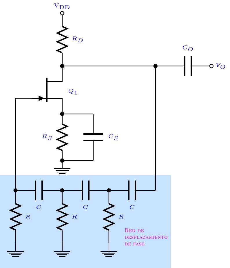
Este ejemplo representa un oscilador de desplazamiento de fase realizado con un transistor JFET Canal-N, dos resistencias y una red de re-alimentación constituida por tres resistencias y tres condensadores idénticos. El condensador CS se utiliza para una configuración de drenaje común y CO permite desacoplar la salida de la red de re-alimentación. Esta red es destacada en un recuadro coloreado de fondo, que se genera usando la biblioteca de TiKZ "backgrounds" Notaciones: Vo = tensión de salida. VDD= polarización positiva en el terminal de drenaje. Todos los componentes eléctricos y electrónicos carecen de valores o tipos. Este esquema es una adaptación de la figura que se encuentra en la página http://www.circuitstoday.com/fet-applications.
Some examples of how the packages tikz and pgfplots can be used to create fully vectorized graphics directly in the LaTeX document. An example of how a flowchart can be generated in LaTeX is also given. It combines the packages tikz and overpic and shows how to overlay/embed intrinsic LaTeX text onto images created elsewhere.
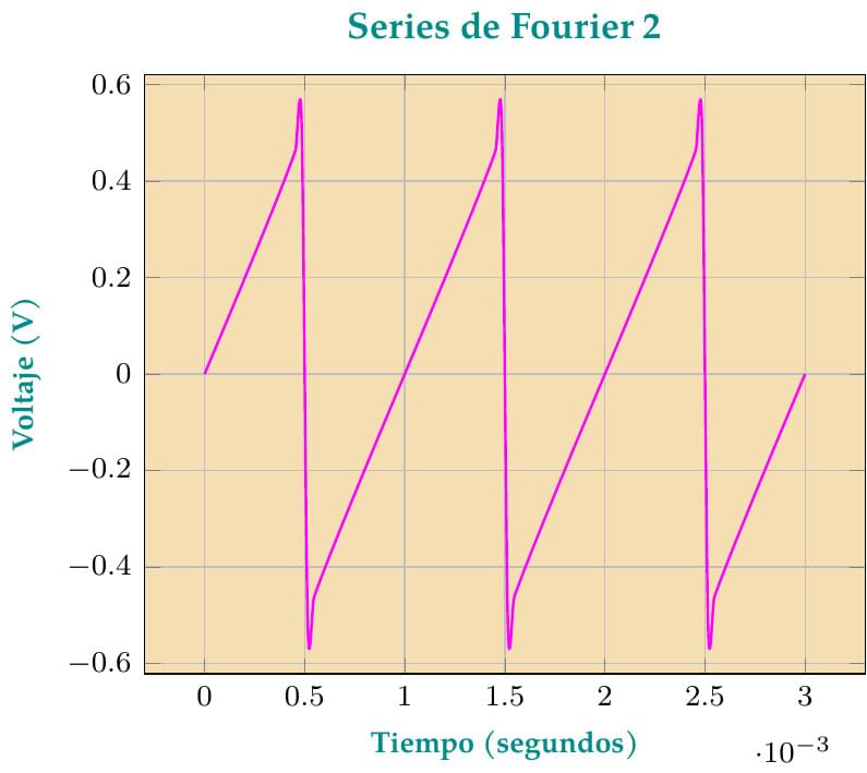
Este gráfico es una mejora, aprovechando el uso de GNUPLOT, de la primera versión que fue publicada por Overleaf. En este caso, la onda de "diente de sierra" es definida según lo indicado en el texto "Mathematical Handbook of Formulas and Tables" de la serie "Schaum's Outlines", de la editorial McGraw Hill, Quinta Edición, página 145. Para mayor precisión, son sumados los 100 primeros términos de la Serie de Fourier, lo cual no afecta grandemente el tiempo de compilación en los servidores de Overleaf.
\begin
Discover why over 25 million people worldwide trust Overleaf with their work.